Priors
Priors on the parameters are set in the beast_settings.txt file using python dictionaries to give the prior model and any related parameters.
All priors are normalized to have an average value of 1. This is possible as the priors are relevant in a relative sense, not absolute and this avoids numerical issues with too large or small numbers.
New prior models can be added in the specific code regions by defining a new prior model name and creating the necessary code to support it. The code files of interest are beast/physicsmodel/prior_weights_[stars,dust].py. New models added should be documented here.
Stellar
Age
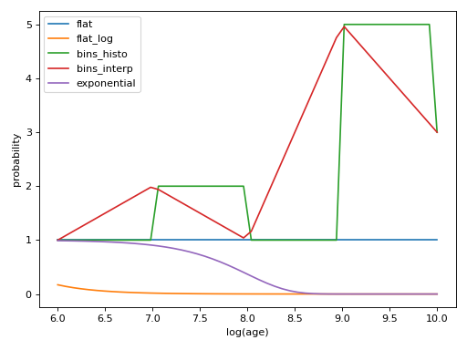
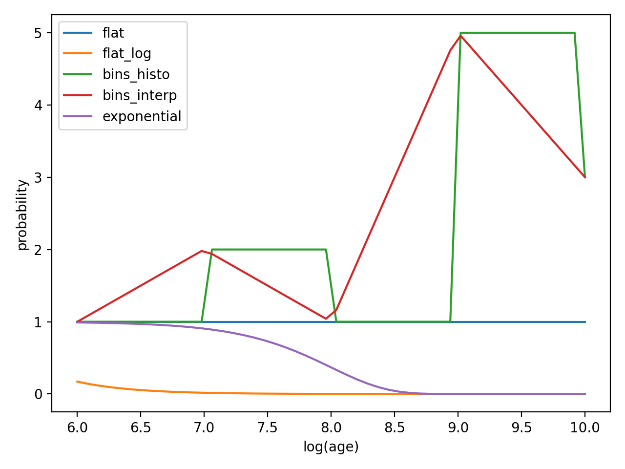
The age prior is the star formation rate (SFR) and can be
Flat in linear age
age_prior_model = {"name": "flat"}
or to set the star formation rate in M_sun/year, use
age_prior_model = {"name": "flat"},
                   "amp": sfr}
Flat in log age
age_prior_model = {"name": "flat_log"}
Set by bins spaced in logage (log10(years)).
For example, step like priors can be specified by:
age_prior_model = {"name": "bins_histo",
                   "x": [6.0, 7.0, 8.0, 9.0, 10.0],
                   "values": [1.0, 2.0, 1.0, 5.0, 3.0]}
Or using bin edges (where N = N_values+1) like those output by np.histogram():
age_prior_model = {"name": "bins_histo",
                   "x": [6.0, 7.0, 8.0, 9.0, 10.0],
                   "values": [1.0, 2.0, 1.0, 5.0]}
For example, lines connecting the bin value of the priors can be specified by:
age_prior_model = {"name": "bins_interp",
                   "x": [6.0, 7.0, 8.0, 9.0, 10.0],
                   "values": [1.0, 2.0, 1.0, 5.0, 3.0]}
4. An exponentially decreasing SFR (in time, but here increasing with age)
with a 0.1 Gyr time constant (with tau parameter in Gyr):
age_prior_model = {"name": "exponential",
                   "tau": 0.1}
Plot showing examples of the possible age prior models with the parameters given above.
(Source code, png, hires.png, pdf)

Mass
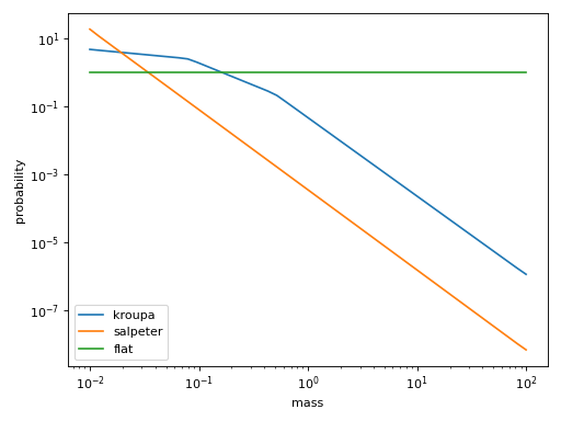
The mass prior is set by the choice of an Initial Mass Function (IMF). The mass function supported are:
Kroupa
Functional form from Kroupa (2001, MNRAS, 322, 231) with alpha0,1,2,3 slopes for <0.08, 0.08-0.5, 0.5-1.0, >1.0 solar masses.
No alpha0,1,2,3 values gives the defaults listed in 2nd example.
mass_prior_model = {"name": "kroupa"}
With explicit values for the alphas (all need to be specified).
mass_prior_model = {"name": "kroupa",
                    "alpha0": 0.3,
                    "alpha1": 1.3,
                    "alpha2": 2.3,
                    "alpha3": 2.3}
Salpeter
Functional form from Salpeter (1955, ApJ, 121, 161).
No slope value gives the default listed in 2nd example.
mass_prior_model = {"name": "salpeter"}
With an explicit value for the slope.
mass_prior_model = {"name": "salpeter",
                    "slope": 2.35}
Flat
There is also a flat mass prior. This is useful for creating grids for BEAST verification (see Simulations), and should not be used for a standard fitting run.
mass_prior_model = {"name": "flat"}
Plot showing examples of the possible mass prior models with the parameters given above.
(Source code, png, hires.png, pdf)
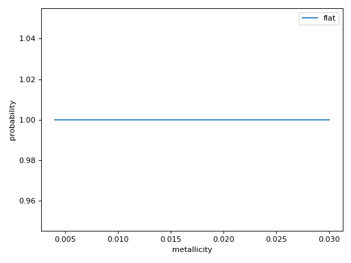
Metallicity
The metallicity prior can be
Flat
met_prior_model = {"name": "flat"}
Plot showing examples of the possible metallicity prior models with the parameters given above.
(Source code, png, hires.png, pdf)
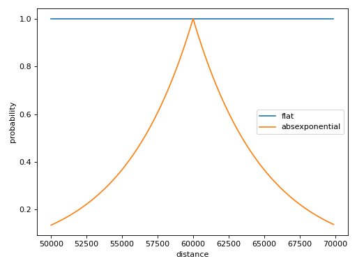
Distance
The distance prior can be
Flat
distance_prior_model = {"name": "flat"}
2. Absolute(Exponential) distribution with an exponential scale height (tau) before and after a fiducial distance (dist0) and an amplitude (amp).
distance_prior_model = {"name": "absexponential",
                        "dist0": 60.0*u.kpc,
                        "tau": 5.*u.kpc,
                        "amp": 1.0}
Plot showing examples of the possible distance prior models with the parameters given above.
(Source code, png, hires.png, pdf)
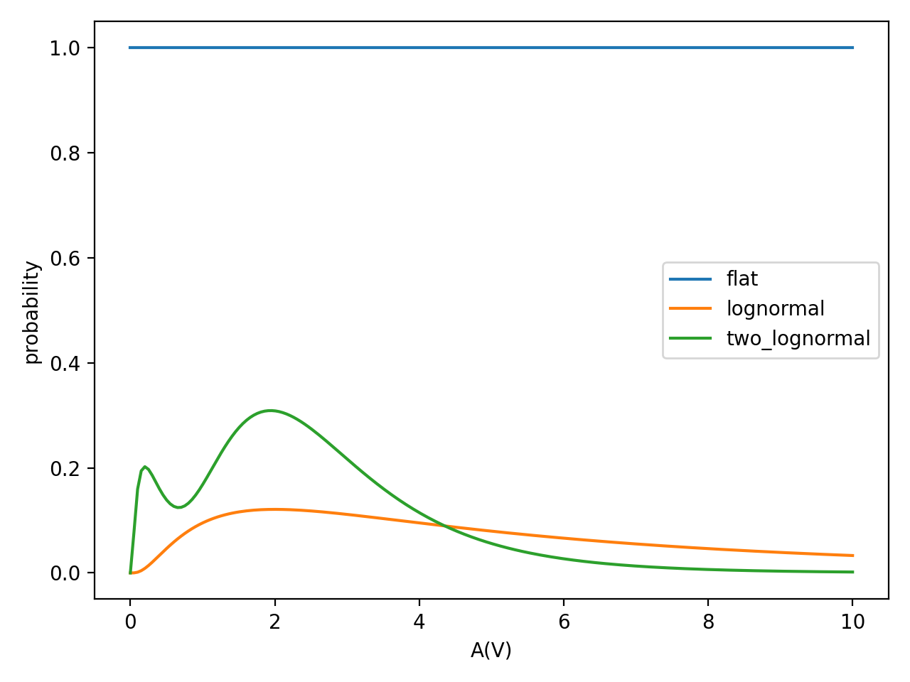
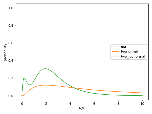
Extinction
A(V)
The A(V) prior can be:
Flat
av_prior_model = {"name": "flat"}
2. Lognormal with the maximum at the A(V) given by mean and the width given by sigma.
av_prior_model = {"name": "lognormal",
                  "mean": 2.0,
                  "sigma": 1.0}
Two lognormals (see above for definition of terms)
av_prior_model = {"name": "two_lognormal",
                  "mean1": 0.2,
                  "mean2": 2.0,
                  "sigma1": 1.0,
                  "sigma2": 0.2,
                  "N1_to_N2": 1.0 / 5.0}
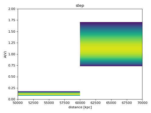
4. Step at a specified distance. Distance must have units. Models the effect of having a dust cloud located at a certain distance. A(V) after dist0 is amp1 + damp2.
av_prior_model = {"name": "step",
                  "dist0": 60 * u.kpc,
                  "amp1": 0.1,
                  "damp2": 1.0,
                  "lgsigma1": 0.05,
                  "lgsigma2": 0.05}
(Source code, png, hires.png, pdf)
(Source code, png, hires.png, pdf)

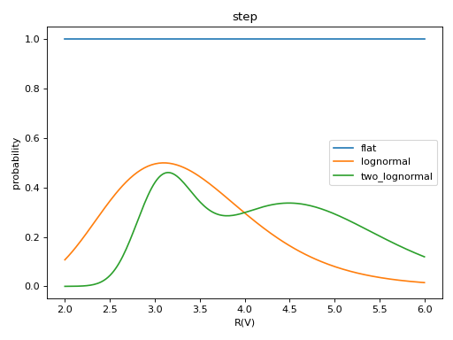
R(V)
Flat
rv_prior_model = {"name": "flat"}
2. Lognormal with the maximum at the R(V) given by mean and the width given by sigma.
rv_prior_model = {"name": "lognormal",
                  "mean": 3.1,
                  "sigma": 0.25}
Two lognormals (see above for definition of terms)
rv_prior_model = {"name": "two_lognormal",
                  "mean1": 3.1,
                  "mean1": 4.5,
                  "sigma1": 0.1,
                  "sigma2": 0.2,
                  "N1_to_N2": 2.0 / 5.0}
4. Step at a specified distance. Distance must have units. Models the effect of having a dust cloud located at a certain distance. R(V) after dist0 is amp1 + damp2.
rv_prior_model = {"name": "step",
                  "dist0": 60 * u.kpc,
                  "amp1": 0.1,
                  "damp2": 1.0,
                  "lgsigma1": 0.05,
                  "lgsigma2": 0.05}
(Source code, png, hires.png, pdf)
(Source code, png, hires.png, pdf)

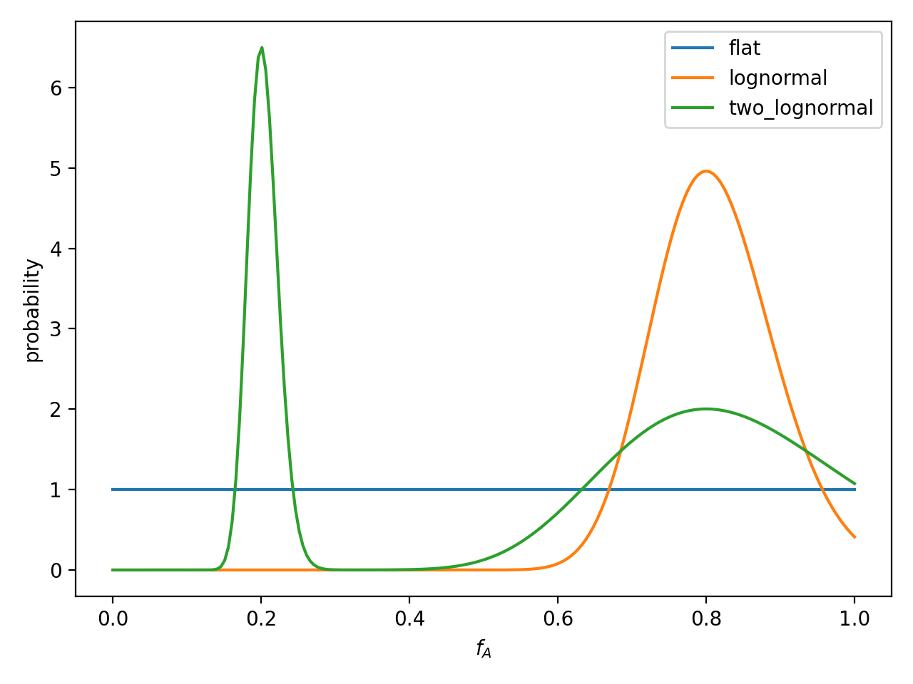
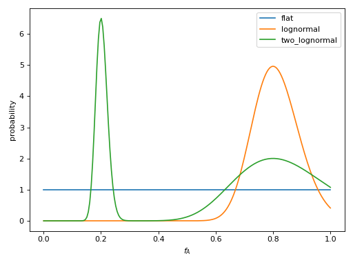
f_A
Flat
fA_prior_model = {"name": "flat"}
2. Lognormal with the maximum at the f_A given by mean and the width given by sigma.
fA_prior_model = {"name": "lognormal",
                  "mean": 0.8,
                  "sigma": 0.1}
Two lognormals (see above for definition of terms)
fA_prior_model = {"name": "two_lognormal",
                  "mean1": 0.1,
                  "mean1": 0.8,
                  "sigma1": 0.1,
                  "sigma2": 0.2,
                  "N1_to_N2": 2.0 / 5.0}
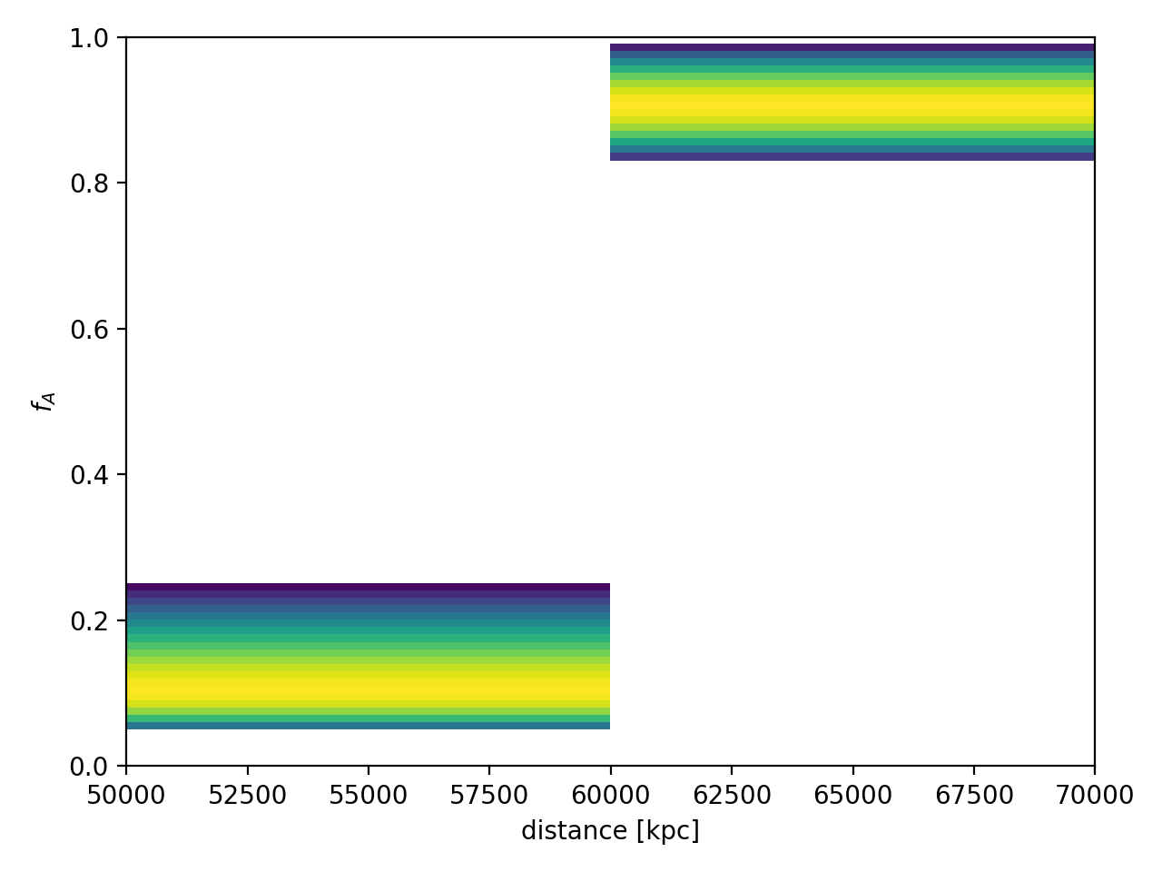
4. Step at a specified distance. Distance must have units. Models the effect of having a dust cloud located at a certain distance. f_A after dist0 is amp1 + damp2.
fA_prior_model = {"name": "step",
                  "dist0": 60 * u.kpc,
                  "amp1": 0.1,
                  "damp2": 0.8,
                  "lgsigma1": 0.1,
                  "lgsigma2": 0.01}
(Source code, png, hires.png, pdf)
(Source code, png, hires.png, pdf)
